お知らせ
過去にQiitaに投稿した内容のアーカイブです。
Timestreamの検索をSDKを使ってやってみました。
クエリーをする最小のコードはこんな感じ。
import boto3
from botocore.config import Config

query = """
    SELECT fleet, truck_id, fuel_capacity, model, load_capacity, make, measure_name, CREATE_TIME_SERIES(time, measure_value::double) as measure
    FROM "IoT-sample"."IoT"
    WHERE measure_value::double IS NOT NULL
    AND measure_name = 'speed'
    GROUP BY fleet, truck_id, fuel_capacity, model, load_capacity, make, measure_name
    ORDER BY fleet, truck_id, fuel_capacity, model, load_capacity, make, measure_name
    LIMIT 2
"""

config = Config(region_name = 'us-east-1')
config.endpoint_discovery_enabled = True
client = boto3.client('timestream-query', config=config)

result = client.query(QueryString=query)
resultはこんな感じ
{
    "QueryId": "AEBQEAMXPVS6RHIUBHJXW6H4BRUINE7GFNEMJMP2AYZFQHAUJLR5ZO4PABHEU2A",
    "Rows": [
        {
            "Data": [
                {
                    "ScalarValue": "Alpha"
                },
                {
                    "ScalarValue": "1234546252"
                },
                {
                    "ScalarValue": "150"
                },
                {
                    "ScalarValue": "W925"
                },
                {
                    "ScalarValue": "1000"
                },
                {
                    "ScalarValue": "Kenworth"
                },
                {
                    "ScalarValue": "speed"
                },
                {
                    "TimeSeriesValue": [
                        {
                            "Time": "2020-10-09 20:53:57.273000000",
                            "Value": {
                                "ScalarValue": "75.0"
                            }
                        },
                        {
                            "Time": "2020-10-09 21:12:02.919000000",
                            "Value": {
                                "ScalarValue": "60.0"
                            }
                        },
                        {
                            "Time": "2020-10-09 21:26:49.334000000",
                            "Value": {
                                "ScalarValue": "10.0"
                            }
                        },
                        {
                            "Time": "2020-10-09 21:31:01.641000000",
                            "Value": {
                                "ScalarValue": "15.0"
                            }
                        },
                        {
                            "Time": "2020-10-09 21:49:01.249000000",
                            "Value": {
                                "ScalarValue": "47.0"
                            }
                        },
                        {
                            "Time": "2020-10-09 21:56:08.380000000",
                            "Value": {
                                "ScalarValue": "44.0"
                            }
                        },
                        {
                            "Time": "2020-10-09 23:50:37.597000000",
                            "Value": {
                                "ScalarValue": "45.0"
                            }
                        },
                        {
                            "Time": "2020-10-10 00:24:09.414000000",
                            "Value": {
                                "ScalarValue": "0.0"
                            }
                        },
                        {
                            "Time": "2020-10-10 00:48:40.046000000",
                            "Value": {
                                "ScalarValue": "55.0"
                            }
                        },
                        {
                            "Time": "2020-10-10 01:33:44.347000000",
                            "Value": {
                                "ScalarValue": "65.0"
                            }
                        }
                    ]
                }
            ]
        },
        {
            "Data": [
                {
                    "ScalarValue": "Alpha"
                },
                {
                    "ScalarValue": "1575739296"
                },
                {
                    "ScalarValue": "100"
                },
                {
                    "ScalarValue": "359"
                },
                {
                    "ScalarValue": "1000"
                },
                {
                    "ScalarValue": "Peterbilt"
                },
                {
                    "ScalarValue": "speed"
                },
                {
                    "TimeSeriesValue": [
                        {
                            "Time": "2020-10-09 21:24:41.479000000",
                            "Value": {
                                "ScalarValue": "17.0"
                            }
                        },
                        {
                            "Time": "2020-10-09 21:51:00.847000000",
                            "Value": {
                                "ScalarValue": "40.0"
                            }
                        },
                        {
                            "Time": "2020-10-09 23:07:10.695000000",
                            "Value": {
                                "ScalarValue": "41.0"
                            }
                        },
                        {
                            "Time": "2020-10-09 23:11:31.029000000",
                            "Value": {
                                "ScalarValue": "60.0"
                            }
                        },
                        {
                            "Time": "2020-10-10 00:03:54.235000000",
                            "Value": {
                                "ScalarValue": "69.0"
                            }
                        },
                        {
                            "Time": "2020-10-10 00:27:58.341000000",
                            "Value": {
                                "ScalarValue": "56.0"
                            }
                        },
                        {
                            "Time": "2020-10-10 00:29:38.188000000",
                            "Value": {
                                "ScalarValue": "4.0"
                            }
                        },
                        {
                            "Time": "2020-10-10 00:30:54.110000000",
                            "Value": {
                                "ScalarValue": "27.0"
                            }
                        },
                        {
                            "Time": "2020-10-10 00:58:07.005000000",
                            "Value": {
                                "ScalarValue": "21.0"
                            }
                        },
                        {
                            "Time": "2020-10-10 01:12:06.518000000",
                            "Value": {
                                "ScalarValue": "30.0"
                            }
                        }
                    ]
                }
            ]
        }
    ],
    "ColumnInfo": [
        {
            "Name": "fleet",
            "Type": {
                "ScalarType": "VARCHAR"
            }
        },
        {
            "Name": "truck_id",
            "Type": {
                "ScalarType": "VARCHAR"
            }
        },
        {
            "Name": "fuel_capacity",
            "Type": {
                "ScalarType": "VARCHAR"
            }
        },
        {
            "Name": "model",
            "Type": {
                "ScalarType": "VARCHAR"
            }
        },
        {
            "Name": "load_capacity",
            "Type": {
                "ScalarType": "VARCHAR"
            }
        },
        {
            "Name": "make",
            "Type": {
                "ScalarType": "VARCHAR"
            }
        },
        {
            "Name": "measure_name",
            "Type": {
                "ScalarType": "VARCHAR"
            }
        },
        {
            "Name": "measure",
            "Type": {
                "TimeSeriesMeasureValueColumnInfo": {
                    "Type": {
                        "ScalarType": "DOUBLE"
                    }
                }
            }
        }
    ],
    "ResponseMetadata": {
        "RequestId": "JRJDO6RN63OVLGZ6ZX52GCCPF4",
        "HTTPStatusCode": 200,
        "HTTPHeaders": {
            "x-amzn-requestid": "JRJDO6RN63OVLGZ6ZX52GCCPF4",
            "content-type": "application/x-amz-json-1.0",
            "content-length": "2413",
            "date": "Sat, 10 Oct 2020 07:33:29 GMT"
        },
        "RetryAttempts": 0
    }
}
result['Rows'][0]['Data'][0]に検索結果が入っています。
そのままではグラフにしづらいので、変形しました。timeがISO 8601形式のUTC時刻で扱いづらいので、datetimeに変換しています。
def convert_callback(x):
    dt = datetime.fromisoformat(x[:26])
    dt = dt.replace(tzinfo= timezone.utc)
    return dt

rows = result['Rows']
for row in rows:
    measure = row['Data'][7]['TimeSeriesValue']

    time = list(map(lambda x: (convert_callback(x['Time'])), measure))
    value = list(map(lambda x: (float(x['Value']['ScalarValue'])), measure))
あとはこいつをグラフにします。
register_matplotlib_converters()
fig = plt.figure()
ax = fig.add_subplot(1, 1, 1)

ax.plot(time, value)

daysFmt = mdates.DateFormatter('%m-%d %H:%M')
ax.xaxis.set_major_formatter(daysFmt)
fig.autofmt_xdate()

plt.show()
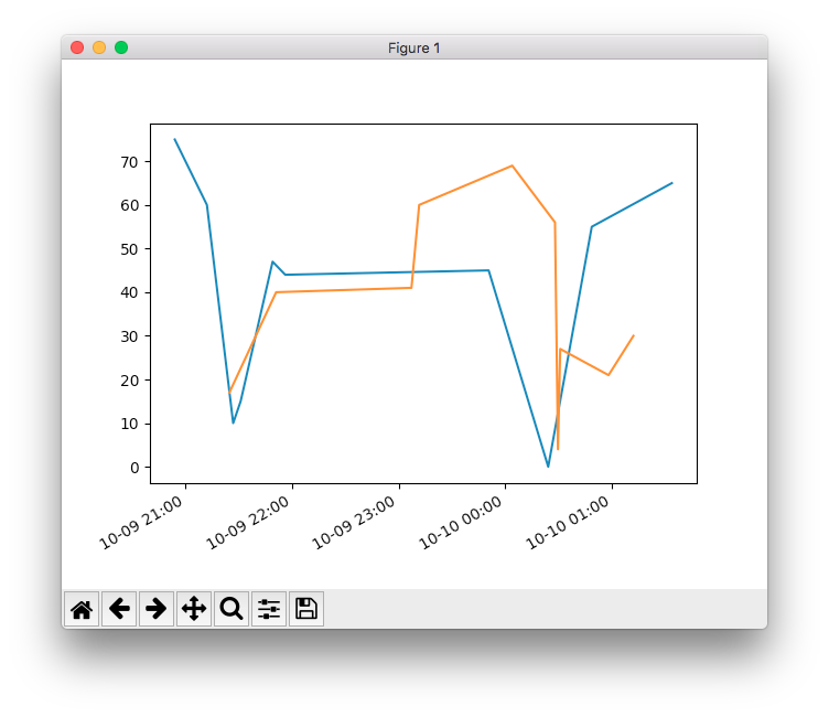
めでたしめでたし。あまり派手なグラフではありませんが。。
コードの全体はこちら。
import json
from datetime import datetime, timezone

import boto3
import matplotlib.dates as mdates
import matplotlib.pyplot as plt
import pandas as pd
from botocore.config import Config
from pandas.plotting import register_matplotlib_converters

query = """
    SELECT fleet, truck_id, fuel_capacity, model, load_capacity, make, measure_name, CREATE_TIME_SERIES(time, measure_value::double) as measure
    FROM "IoT-sample"."IoT"
    WHERE measure_value::double IS NOT NULL
    AND measure_name = 'speed'
    GROUP BY fleet, truck_id, fuel_capacity, model, load_capacity, make, measure_name
    ORDER BY fleet, truck_id, fuel_capacity, model, load_capacity, make, measure_name
    LIMIT 2
"""

def create_client():
    config = Config(region_name = 'us-east-1')
    config.endpoint_discovery_enabled = True
    client = boto3.client('timestream-query', config=config)
    return client

def convert_callback(x):
    dt = datetime.fromisoformat(x[:26])
    dt = dt.replace(tzinfo= timezone.utc)
    return dt

if __name__ == "__main__":

    client = create_client()
    result = client.query(QueryString=query)

    rows = result['Rows']

    register_matplotlib_converters()
    fig = plt.figure()
    ax = fig.add_subplot(1, 1, 1)

    for row in rows:
        measure = row['Data'][7]['TimeSeriesValue']

        time = list(map(lambda x: (convert_callback(x['Time'])), measure))
        value = list(map(lambda x: (float(x['Value']['ScalarValue'])), measure))

        ax.plot(time, value)

    daysFmt = mdates.DateFormatter('%m-%d %H:%M')
    ax.xaxis.set_major_formatter(daysFmt)
    fig.autofmt_xdate()

    plt.show()